Watch on YouTube - Video notes - Full video and playlist - Infinite Sequences and Series playlist
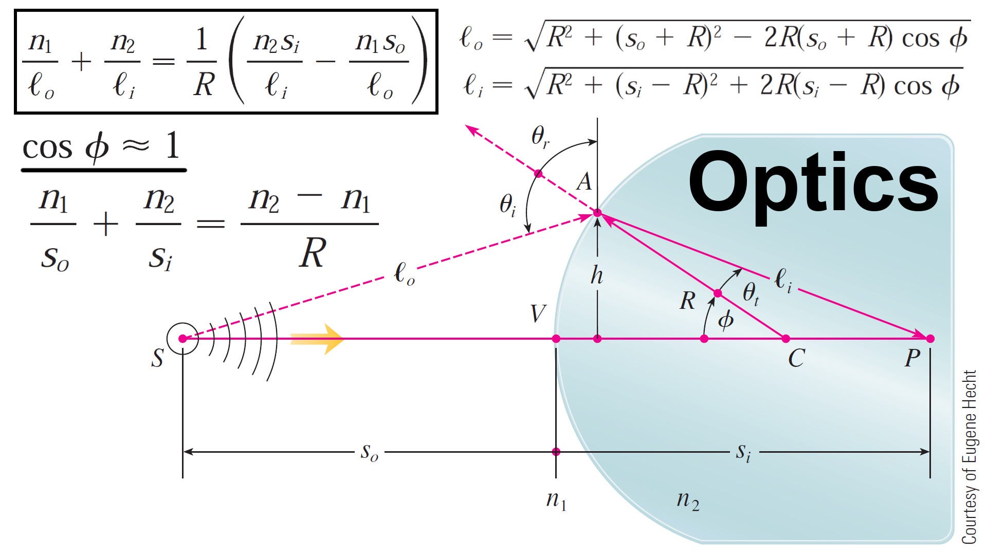
In this video, I demonstrate how Taylor polynomials are used in optical physics to simplify the complex refraction equation. The refraction path lengths of light outside and inside a refractive medium, like a glass lens, can be derived using the Law of Cosines. However, the resulting equation is often cumbersome to work with. In first-order optics, we approximate these lengths using the first-order Taylor polynomial for cosine, where cos(x) is approximated as 1. For larger angles, a more accurate approximation is needed, so we use the third-degree Taylor polynomial instead, a method known as third-order optics.
Timestamps:
Example 2: Error approximation for sin(x) Taylor polynomials: 0:00
Solution to (a): Maclaurin series for sin(x): 0:41
Maclaurin sine series is alternating when x is not zero: 2:03
Can use Alternating Series Estimation Theorem to calculate the error: 5:02
Absolute value of error is less than 4.3x10^(-8): 7:56
Approximating sin(12 degrees) by converting to radians first: 9:41
sin(12°) = 0.207912 correct to 6 decimal places: 13:09
Solution to (b): Values of x to have accuracy less than 0.0005: 15:28
Accuracy is within 0.0005 for when the absolute value of x is less than 0.82: 18:55
Example 2 using Taylor's Inequality: 20:27
Solving for 7th derivative of sin(x): 22:10
Taylor's Inequality gives same result as the Alternating Estimation Theorem: 23:52
Graphing the Remainder Function with Desmos: https://www.desmos.com/calculator/yphi6wpizp: 27:24
Error is less than 4.3x10^(-8) just as in Part (a): 29:49
Graphing Remainder function and y = 0.00005 in Desmos: https://www.desmos.com/calculator/5uuyhdlp1y: 30:58
Interval of error is between absolute of x less than 0.82 just like in part (b): 31:48
For different angles we can use Taylor Polynomials centered at different values of x: 32:56
Graphing various Maclaurin polynomials for sin(x) using Desmos: https://www.desmos.com/calculator/8pl3nc2zha: 33:33
The Maclaurin polynomial with the most terms is the most accurate: 35:22
Taylor Polynomials are used in Calculators and Computers to solve functions like sine and e^x: 36:58